Building a Machine Learning Data Pipeline with Gridscript: From JSON and CSV to Machine Learning Model
Data pipelines are the foundation of modern analytics and machine learning workflows. With gridscript.io, you can connect multiple data sources, clean and transform your data, and seamlessly integrate Python and scikit-learn - all inside one visual, reproducible environment. In this tutorial, you'll create a simple yet powerful Gridscript pipeline that predicts whether employees will leave a company based on HR, payroll, and satisfaction data.
Scenario
You have three datasets:
- A JSON file with employee info
- A CSV file with payroll data
- An XLSX file with satisfaction survey results
Your goal:
- Merge all sources
- Clean and enrich the data
- Train a simple Logistic Regression model using scikit-learn
Sample Data
employees.json
[
  {"employee_id": 1, "name": "Alice", "department": "Engineering", "years_at_company": 3, "left_company": 0},
  {"employee_id": 2, "name": "Bob", "department": "Sales", "years_at_company": 2, "left_company": 1},
  {"employee_id": 3, "name": "Charlie", "department": "Engineering", "years_at_company": 5, "left_company": 0},
  {"employee_id": 4, "name": "Diana", "department": "HR", "years_at_company": 4, "left_company": 1},
  {"employee_id": 5, "name": "Ethan", "department": "Marketing", "years_at_company": 1, "left_company": 0}
]
payroll.csv
employee_id,salary,bonus
1,85000,5000
2,62000,2000
3,90000,7000
4,55000,1500
5,60000,3000
satisfaction.xlsx
employee_id	satisfaction_score
1	         0.8
2                0.4
3	         0.9
4	         0.3
5	         0.6
Step 1: Load and Merge Data
In your Gridscript pipeline, create three “Import” stages as follows:

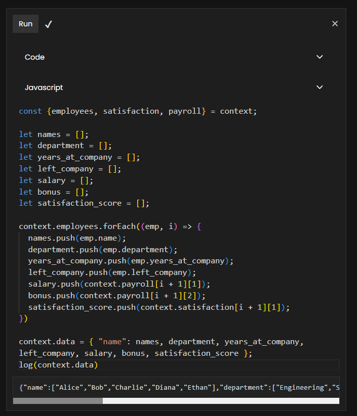
Then create a Code stage to merge the data together (I will use JavaScript for this example but you can go ahead and use Python if you prefer it):
const {employees, satisfaction, payroll} = context;

let names = [];
let department = [];
let years_at_company = [];
let left_company = [];
let salary = [];
let bonus = [];
let satisfaction_score = [];

context.employees.forEach((emp, i) => {
  names.push(emp.name);
  department.push(emp.department);
  years_at_company.push(emp.years_at_company);
  left_company.push(emp.left_company);
  salary.push(context.payroll[i + 1][1]);
  bonus.push(context.payroll[i + 1][2]);
  satisfaction_score.push(context.satisfaction[i + 1][1]);
})

context.data = {
    "name": names,
    department,
    years_at_company,
    left_company,
    salary,
    bonus,
    satisfaction_score
};
log(context.data)
This is the result that we get from running the previous stage:
{
    "name":["Alice","Bob","Charlie","Diana","Ethan"],
    "department":["Engineering","Sales","Engineering","HR","Marketing"],
    "years_at_company":[3,2,5,4,1],
    "left_company":[0,1,0,1,0],
    "salary":[85000,62000,90000,55000,60000],
    "bonus":[5000,2000,7000,1500,3000],
    "satisfaction_score":[0.8,0.4,0.9,0.3,0.6]
}
Step 2: Clean and Transform Data
Once the raw data has been merged into a single unified table, the next step is data cleaning and feature engineering. This is where we convert all values into a modeling-friendly format and create new features that may improve model performance.
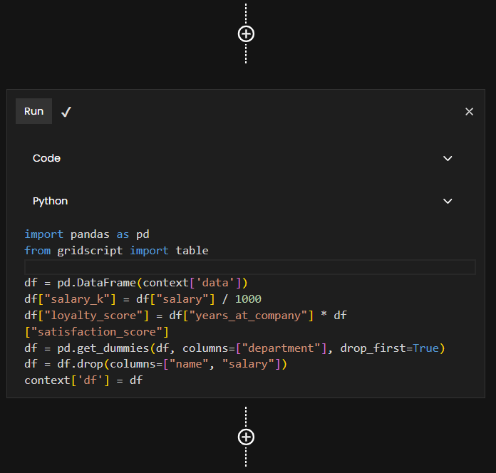
In Gridscript, we can do this using a Python code stage. The code below performs several important preprocessing steps:
import pandas as pd
from gridscript import table

df = pd.DataFrame(context['data'])
df["salary_k"] = df["salary"] / 1000
df["loyalty_score"] = df["years_at_company"] * df["satisfaction_score"]
df = pd.get_dummies(df, columns=["department"], drop_first=True)
df = df.drop(columns=["name", "salary"])
context['df'] = df
What’s happening here?
-
Converting raw salary to salary_k: Machine learning models often work better when numerical values are in a similar range. Dividing salary by 1,000 makes the feature easier to learn from and easier to interpret.
-
Creating a new feature loyalty_score:
years_at_company × satisfaction_scoregives a simple proxy for engagement or stability. Someone who has been at the company 5 years with a 0.9 satisfaction score is likely much more loyal than someone who has been there 1 year with 0.3 satisfaction. Feature engineering like this often boosts predictive performance. -
One-hot encoding the department column: Machine learning algorithms can't directly understand text categories (like "Engineering" or "HR").
pd.get_dummies()converts each department into a binary (0/1) column. Usingdrop_first=Trueavoids multicollinearity by removing one reference category. -
Removing unnecessary columns: name is not useful for prediction and salary is replaced by the cleaner
salary_k.
Result
After this transformation, every column in df is numeric, making it fully ready for machine learning in the next stage.
Step 3: Prepare Features and Train a Logistic Regression Model
Now that the dataset is clean and numeric, it’s time to train a machine learning model.
In this example, we use Logistic Regression, one of the most common algorithms for binary classification problems like predicting employee attrition (left_company).
from sklearn.model_selection import train_test_split
from sklearn.preprocessing import StandardScaler
from sklearn.linear_model import LogisticRegression
from sklearn.pipeline import Pipeline
from sklearn.metrics import accuracy_score, confusion_matrix
import pandas as pd

scaler = StandardScaler()
X_scaled = scaler.fit_transform(X)

df = pd.DataFrame(context["df"])

# Separate features and target
X = df.drop(columns=["left_company"])
y = df["left_company"]

# Full Pipeline: scale numeric features + logistic regression
model = Pipeline(steps=[
    ("scaler", StandardScaler()),
    ("classifier", LogisticRegression())
])

# Split the data
X_train, X_test, y_train, y_test = train_test_split(
    X, y, test_size=0.2, random_state=42
)

# Train
model.fit(X_train, y_train)

# Predict
preds = model.predict(X_test)

# Results
print("Predictions:", preds)
print("Accuracy:", accuracy_score(y_test, preds))
print("Confusion Matrix:\n", confusion_matrix(y_test, preds))
Explanation of Step 3
- Separating features (
X) from the target (y):Xcontains the variables used to make a prediction,ycontains 0 or 1 — whether the employee left the company. This is standard practice in machine learning. - Using a Pipeline: The pipeline bundles preprocessing and model training into one reproducible sequence.
- Splitting the dataset (train/test split): 80% of the data is used to train the model, 20% is kept unseen to test how well the model generalizes, this is essential to avoid overfitting.
- Evaluating the model, the code outputs: Predictions, Accuracy — percentage of correct predictions, Confusion matrix — how many 0s and 1s were classified correctly or incorrectly.
This gives you a quick understanding of the model’s performance.

Step 4: Run It All as a Gridscript Pipeline
Now that each stage works, you can chain them visually inside Gridscript.io to build a fully reproducible end-to-end data pipeline.
A typical Gridscript pipeline for this project looks like this:
- Import the JSON, CSV, and XLSX datasets
- Merge Data
- Clean & Transform Data
- Engineer features
- Create, Train & Evaluate Model
Why This Example Works
This example demonstrates how Gridscript pipelines:
- Integrate multiple data sources (JSON, CSV, XLSX)
- Perform data transformation and feature engineering
- Enable machine learning workflows with scikit-learn
- Make your process reproducible and shareable
Pipeline Features
- Reproducibility: Every stage is versioned and saved. If new data arrives, you just rerun the pipeline — no code changes needed.
- Transparency: You can inspect outputs at each stage. This makes debugging and experimentation far easier than writing a monolithic script.
- Modularity: Want to try A RandomForestClassifier? A different set of features? A new data source? Just swap in or duplicate a stage — the rest of the pipeline stays intact.
- Collaboration: Teams can share pipelines, comment on steps, and review changes — ideal for data scientists, analysts, and ML engineers.
Next Steps
Try extending the pipeline by:
- Adding more features (e.g., bonus/salary ratio)
- Trying a RandomForestClassifier
- Visualizing feature importance in another Gridscript cell
Try now Gridscript pipelines here.